Graphs - Aug. and Training
Summary of GNN lectures
GNN Augmentation and Training#
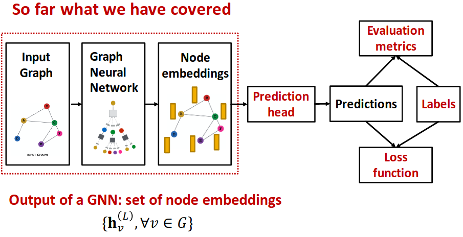
GNN Training Pipeline#
e.g.: Latin exempli gratia (for example)
Prediction Head#
Different task levels require different prediction heads
Node-level prediction#
- After GNN computation, we have -dim node embeddings:
- Suppose we want to make -way prediction (Classification, Regression)
- ;
Edge-level prediction#
;
;
(1-way prediction (e.g., predict the existence of an edge))
Applying to -way prediction:
Graph-level prediction#
is possible in .
But! Simple global pooling over a (large) graph will lose information.
- A solution: Let’s aggregate all the node embeddings hierarchically
DiffPool#
Ying et al., Hierarchical Graph Representation Learning with Differentiable Pooling
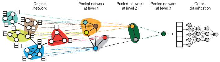
- Hierarchically pool node embeddings
- Leverage 2 independent GNNs at each level
- GNN A: Compute node embeddings
- GNN B: Compute the cluster that a node belongs to
- GNNs A and B at each level can be executed in parallel
- For each Pooling layer
- Use clustering assignments from GNN B to aggregate node embeddings generated by GNN A
- Create a single new node for each cluster, maintaining edges between clusters to generated a new pooled network
- Jointly train GNN A and GNN B
Training#
Supervised learning
Labels come from external sources
- Node labels : in a citation network, which subject area does a node belong to
- Edge labels : in a transaction network, whether an edge is fraudulent
- Graph labels : among molecular graphs, the drug likeness of graphs
Advice: Reduce your task to node / edge / graph labels, since they are easy to work with
e.g., We knew some nodes form a cluster. We can treat the cluster that a node belongs to as a node labelUnsupervised learning (Self-supervised learning)
we can find supervision signals within the graph.
- Node-level : Such as clustering coefficient, PageRank, …
- Edge-level : Hide the edge between two nodes, predict if there should be a link
- Graph-level : For example, predict if two graphs are isomorphic
Sometimes the differences are blurry
- We still have “supervision” in unsupervised learning
- e.g., train a GNN to predict node clustering coefficient
- An alternative name for “unsupervised” is “self-supervised”
Data Splitting#
Transductive setting: The entire graph can be observed in all dataset splits, we only split the labels
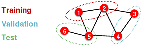
- At training time, we compute embeddings using the entire graph, and train using node 1&2’s labels
- At validation time, we compute embeddings using the entire graph, and evaluate on node 3&4’s labels
- Only applicable to node / edge prediction tasks
- (training / validation / test) sets are on the same graph
Inductive setting: Each split can only observe the graph(s) within the split, we break the edges between splits to get multiple graphs. A successful model should generalize to unseen graphs.
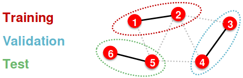
- At training time, we compute embeddings using the graph over node 1&2, and train using node 1&2’s labels
- At validation time, we compute embeddings using the graph over node 3&4, and evaluate on node 3&4’s labels
- Applicable to node / edge / graph tasks
- (training / validation / test sets) are on different graphs
Data Splitting in Tasks#
- Node Classification
- Transductive node classification
- Inductive node classification
- Graph Classification
- Only the inductive setting is well defined for graph classification
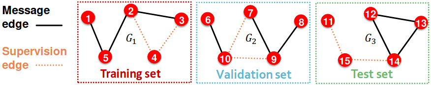
- Link Prediction
- Assign 2 types of edges in the original graph
- Message edges: Used for GNN message passing
- Supervision edges: Use for computing objectives (will not be fed into GNN)
- Split edges into train / validation / test
Option 1: Inductive link prediction split
Option 2: Transductive link prediction split
- By definition of “transductive”, the entire graph can be observed in all dataset splits
- But since edges are both part of graph structure and the supervision, we need to hold out validation / test edges
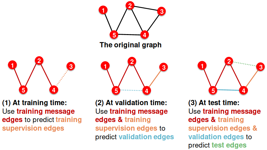
- Assign 2 types of edges in the original graph
- previous Graphs - Neural Networks
- next Graphs - Theory