• CS224W: Machine Learning with Graphs

Graph Neural Networks#

Limitations of Shallow embedding methods#

Embedding matrix $\bf Z$, It’s shape. (dim. of embds, # nodes)

• $O(|V|d)$ parameters are needed:
  • No sharing of parameters between nodes
  • Every node has its own unique embedding
• Inherently “transductive”:
  • Cannot generate embeddings for nodes that are not seen during training
• Do not incorporate node features:
  • Nodes in many graphs have features that we can and should leverage

Graph#

$\text{ENC}$: multiple layers of non-linear transformations based on graph structure

Tasks we will be able to solve:

• Node classification: Predict the type of a given node
• Link prediction: Predict whether two nodes are linked
• Community detection: Identify densely linked clusters of nodes
• Network similarity: How similar are two (sub)networks

Graph networks are more complex than images or text. (Arbitray size, complex topological structure)

Fundamental Func.
$\Theta^* \larr \Theta - \eta\nabla_{\Theta}{\cal L}$

Adjacency matrix를 linear layer에 그대로 넣게 되면, linear layer의 weight들은 node order에 민감하여, 순서가 변경되면 매우 다른 값을 가지게 된다. 또한 $O(|V|)$ paramters를 가지게 되고, 고정된 feature dim으로 다른 크기의 graph를 사용할 수 없다.

Graph does not have a canonical order of the nodes!

Graph is permutation invariant

${\bf X} \in {\Bbb R}^{|V|\times d}$ is a matrix of node features.

Permutation Invariant#

Then, if $f({\bf A}_i, {\bf X}_i) = f({\bf A}_j, {\bf X}_j)$ for any order plan $i$ and $j$, we formally say $f$ is a permutation invariant function.

• Definition: For any graph function $f: {\Bbb R}^{|V|\times m}\times {\Bbb R}^{|V|\times|V|} \rarr {\Bbb R}^d$, $f$ is permutation-invariant if $f({\bf A},{\bf X}) = f({\bf PAP^\top}, {\bf PX})$ for any permutation $\bf P$.
• Permute the input, the output stays the same. (map a graph to a vector)
• e.g. $f$: sum, average, pooling

Permutation Equivariance#

If the output vector of a node at the same position in the graph remains unchanged for any order plan, we say $f$ is permutation equivariant.

• Definition: For any node function $f: {\Bbb R}^{|V|\times m}\times {\Bbb R}^{|V|\times|V|} \rarr {\Bbb R}^{|V|\times m}$, $f$ is permutation-equivariant if ${\bf P}f({\bf A},{\bf X}) = f({\bf PAP^\top}, {\bf PX})$ for any permutation $\bf P$.
• Permute the input, output also permutes accordingly. (map a graph to a matrix)
• e.g. $f$: RNN, Self-attention

Examples:

1. $f({\bf A},{\bf X}) = {\bf 1^\top X}$: Permutation-invariant
   $\rarr f({\bf PAP^\top}, {\bf PX}) = {\bf 1^\top PX} = {\bf 1^\top X} = f({\bf A}, {\bf X})$
2. $f({\bf A},{\bf X}) = {\bf X}$: Permutation-equivariant
   $\rarr f({\bf PAP^\top}, {\bf PX}) = {\bf PX} = {\bf P}f({\bf A}, {\bf X})$
3. $f({\bf A},{\bf X}) = {\bf AX}$: Permutation-equivariant
   $\rarr f({\bf PAP^\top}, {\bf PX}) = {\bf PAP^\top PX} = {\bf PAX} = {\bf P}f({\bf A}, {\bf X})$

Graph Convolutional Networks#

Idea: Node’s neighborhood defines a computation graph

cs224w - lecture 4. slide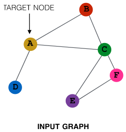

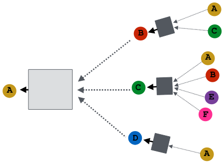
Intuition: Nodes aggregate information from their neighbors using neural networks

Model can be of arbitrary depth.

Neighborhood Aggregation#

Neighborhood aggregation: Key distinctions are in how different approaches aggregate information across the layers

Basic approach.

$\begin{aligned}
&{\rm h}_v^0={\rm x}_v\\
&{\rm h}_v^{(k+1)}=\sigma\left({\rm W}_k\sum_{u\in{\rm N}(v)}\frac{{\rm h}_u^{(k)}}{|{\rm N}(v)|}+{\rm B}_k{\rm h}_v^{(k)}\right),\ \forall k\in\{0,\ \dots,\ {\small K-1}\}\\
&{\rm z}_v={\rm h}_v^{(K)}
\end{aligned}$

${\rm h}_v^0$: Initial 0th layer embeddings are equal to node features.
$\sigma$: Non-linearity activation function.
$\sum_{u\in{\rm N}(v)}\frac{{\rm h}_u^{(k)}}{|{\rm N}(v)|}$: Average of neighbor’s previous layer embeddings.
${\rm h}_v^{(k)}$: Embedding of $v$ at layer $k$
${\rm z}_v$: Embedding after K layers of neighborhood aggregation
${\rm W}_k$: weight matrix for neighborhood aggregation
${\rm B}_k$: weight matrix for transforming hidden vector of self

GCN: Invariance and Equivariance#

Given a node, the GCN that computes its embedding is permutation invariant.

Average of neighbor’s previous layer embeddings - Permutation invariant.
(Average 때문 순서 상관 없다)

Considering all nodes in a graph, GCN computation is permutation equivariant.

cs224w - lecture 4. slide

• Let ${\rm H}^{(k)} = [h_1^{(k)},\ \dots,\ h_{|V|}^{(k)}]^\top$, then $\sum_{u\in N_v} h_u^{(k)}={\rm A}_v{\rm H^{(k)}}$
• Diagonal matrix ${\rm D}$
  • ${\rm D}_{v,v} = \deg(v)= |N(v)|,\ {\rm D}_{v,v}^{-1} = \frac{1}{|N(v)|}$
• Therefore, $\sum_{u\in N(v)}\frac{{\rm h}_u^{(k)}}{|N(v)|}$ is ${\rm H}^{(k+1)} = {\rm D^{-1}AH}^{(k)}$.

${\rm H}^{(k+1)}=\sigma\left({\rm \tilde{A}}{\rm H}^{(k)}{\rm W}_k^\top + {\rm H}^{(k)}{\rm B}_k^\top \right)$

$\rm \tilde{A} = D^{-1}A$

How to Train a GNN#

Supervised setting#

Node label available

${\cal L}=\sum_{v\in V}\text{CE}(y_{v},\sigma({\rm z}_v^\top\theta))$

${\rm z}_v^\top$: Encoder output
$y_v$: Node class label
$\theta$: Classification weights

Unsupervised setting#

No node label available

Use the graph structure as the supervision!

${\cal L}=\sum_{z_u, z_v}\text{CE}(y_{u,v},\text{DEC}(z_u,z_v))$

“Similar” nodes have similar embeddings

$\text{DEC}$ is the decoder such as inner product.

Model Process#

1. Define a neighborhood aggregation
2. Define a loss function on the embeddings
3. Train on a set of nodes, i.e., a batch of compute graphs
4. Generate embeddings for nodes as needed (Only compute the relevant nodes in the batch.)

Inductive Capability: New Nodes and New Graphs#

The same aggregation parameters are shared for all nodes:

• The number of model parameters is sublinear in $|V|$ and we can generalize to unseen nodes!

Inductive node embedding –> Generalize to entirely unseen graphs

A General Perspective on GNN#

A General GNN Framework#

cs224w - lecture 5. slide

1. Message
2. Aggregation
3. Layer connectivity
4. Graph augmentation
   Idea: Raw input graph $\neq$ Computational graph
   • Graph feature augmentation
   • Graph structure augmentation
5. Learning objective

A Single Layer of a GNN#

Idea of a GNN Layer: Compress a set of vectors into a single vector

Message#

Message function: Each node will create a message, which will be sent to other nodes later.

${\rm m}_u^{(l)} = \text{\small MSG}^{(l)}({\rm h}_u^{(l
-1)})$

If message function($\text{MSG}$) is a linear layer, ${\rm m}_u^{(l)} = {\rm W}^{(l)}{\rm h}_u^{(l-1)}$

Aggregation#

Intuition: Each node will aggregate the messages from node $v$’s neighbors

${\rm h}_u^{(l)} = \text{\small AGG}^{(l)}(\{{\rm m}_u^{(l)},u\in N(v)\})$

Possible aggregation functions, $\text{sum}(\cdot),\ \text{mean}(\cdot),\ \text{max}(\cdot)$

Issue: Information from node $v$ itself could get lost

• message 내에 포함된 정보는 자신을 제외한 $v$ 이웃 노드들의 정보만 가지고 있기 때문이다.

Solution:

1. Compute message from node $v$ itself.
   ${\rm m}_v^{(l)} = {\rm B}^{(l)}{\rm h}_v^{(l-1)}$
2. ${\rm h}_v^{(l)} = \text{\small CONCAT}(\text{\small AGG}^{(l)}(\{{\rm m}_u^{(l)},u\in N(v)\}), {\rm m}_v^{(l)})$

Finally,

1. Message: ${\rm m}_u^{(l)} = \text{\small MSG}^{(l)}({\rm h}_u^{(l-1)}), u \in \{N(v)\cup v\}$
2. Aggregation: ${\rm h}_v^{(l)} = \text{\small AGG}^{(l)}(\{{\rm m}_u^{(l)},u\in N(v)\}, {\rm m}_v^{(l)})$

Classical GNN Layers#

Recap: a single GNN layer

Graph Convolutional Networks (GCN)#

${\rm h}_v^{(l)}=\sigma\left({\rm W}^{(l)}\sum_{u\in{\rm N}(v)}\frac{{\rm h}_u^{(l-1)}}{|{\rm N}(v)|}\right)$

1. ${\rm m}_u^{(l)} = \frac{1}{|N(v)|}{\rm W}^{(l)}{\rm h}_u^{(l-1)}$
2. ${\rm h}_v^{(l)} = \sigma(\text{sum}(\{{\rm m}_u^{(l)},u\in N(v)\}))$

GraphSAGE#

${\rm h}_v^{(l)} = \sigma\left({\rm W}^{(l)}\cdot\text{\small CONCAT}\left(\text{\small AGG}(\{{\rm h}_u^{(l-1)},\forall u\in N(v)\}), {\rm h}_v^{(l-1)}\right)\right)$

1. Message is computed within the $\text{AGG}(\cdot)$
2. Two-stage aggregation
   1. ${\rm h}_{N(v)}^{(l)}\larr \text{\small AGG}(\{{\rm h}_u^{(l-1)},\forall u\in N(v)\})$
   2. ${\rm h}_{v}^{(l)}\larr \sigma\left({\rm W}^{(l)}\cdot\text{\small CONCAT}\left({\rm h}_{N(v)}^{(l)}, {\rm h}_v^{(l-1)}\right)\right)$

Neighbor aggregation methods#

1. Mean: Take a weighted average of neighbors
   $\text{\small AGG} = \sum_{u\in{\rm N}(v)}\frac{{\rm h}_u^{(l-1)}}{|{\rm N}(v)|}$
2. Pool: Transform neighbor vectors and apply symmetric vector function $\text{mean}(\cdot)$ or $\text{max}(\cdot)$
   $\text{\small AGG} = \text{\small mean}(\{\text{\small MLP}({\rm h}_u^{(l-1)}),\forall u\in N(v)\})$
3. LSTM: Apply LSTM to reshuffled of neighbors
   $\text{\small AGG} = \text{\small LSTM}([{\rm h}_u^{(l-1)},\forall u\in \pi(N(v))])$

${\ell}_2$ Normalization#

${\rm h}_v^{(l)} \larr \frac{{\rm h}_v^{(l)}}{{\|{\rm h}_v^{(l)}\|}_2}, \forall v\in V$ where ${\|u\|}_2 = \sqrt{\sum_i u_i^2}$

Graph Attention Networks#

${\rm h}_v^{(l)} = \sigma\left(\sum_{u\in N(v)}\alpha_{vu}{\rm W}^{(l)}{\rm h}_u^{(l-1)}\right)$

In GCN and GraphSAGE:

• $\alpha_{vu} = \frac{1}{|N(v)|}$ is weighting factor (importance) of node $u$’s message to node $v$.
• $\alpha_{vu}$ is defined explicitly based on the structural properties of the graph (node degree).
• All neighbors $u \in N(v)$ are equally important to node $v$.

Goal: Specify arbitrary importance to different neighbors of each node in the graph

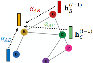
Idea: Compute embedding ${\rm h}_v^{(l)}$ of each node in the graph following an attention strategy:

• Nodes attend over their neighborhoods’ message
• Implicitly specifying different weights to different nodes in a neighborhood

Attention Mechanism#

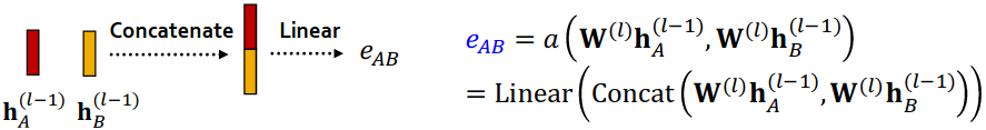
Let $\alpha_{vu}$ be computed as a byproduct of an attention mechanism $a$:

1. Let $a$ compute attention coefficients $e_{vu}$ across pairs of nodes $u$, $v$ based on their messages:

   $e_{vu} = a({\rm W}^{(l)}{\rm h}_u^{(l-1)},{\rm W}^{(l)}{\rm h}_v^{(l-1)})$

2. Normalize with softmax

   $\alpha_{vu} = \frac{\exp(e_{vu})}{\sum_{k\in N(v)}\exp(e_{vk})}$

3. Weighted sum based on the final attention weight $\alpha_{vu}$

   cs224w - lecture 5. slide

   $\begin{aligned}
    {\rm h}_A^{(l)} = \sigma(
    &\alpha_{\text{AB}}{\rm W}^{(l)}{\rm h}_\text{B}^{(l-1)}\\
    &+\alpha_{\text{AC}}{\rm W}^{(l)}{\rm h}_\text{C}^{(l-1)}\\
    &+\alpha_{\text{AD}}{\rm W}^{(l)}{\rm h}_\text{D}^{(l-1)})
    \end{aligned}$

What is the form of attention mechanism $a$?

The approach is agnostic to the choice of $a$

• Simple example

  cs224w - lecture 5. slide

Multi-head attention#

Stabilizes the learning process of attention mechanism
(하나의 head로만은 bias 되기 쉽다.)

1. ${\rm h}_v^{(l)}[1] = \sigma\left(\sum_{u\in N(v)}\alpha_{vu}^1{\rm W}^{(l)}{\rm h}_u^{(l-1)}\right)$
   ${\rm h}_v^{(l)}[2] = \sigma\left(\sum_{u\in N(v)}\alpha_{vu}^2{\rm W}^{(l)}{\rm h}_u^{(l-1)}\right)$
   ${\rm h}_v^{(l)}[3] = \sigma\left(\sum_{u\in N(v)}\alpha_{vu}^3{\rm W}^{(l)}{\rm h}_u^{(l-1)}\right)$

2. ${\rm h}_v^{(l)} = \text{\small AGG}({\rm h}_v^{(l)}[1],{\rm h}_v^{(l)}[2],{\rm h}_v^{(l)}[3])$

Key benefit: Allows for (implicitly) specifying different importance values ($\alpha_{vu}$) to different neighbors

• Computationally efficient:
  • Computation of attentional coefficients can be parallelized across all edges of the graph
  • Aggregation may be parallelized across all nodes
• Storage efficient:
  • Sparse matrix operations do not require more than $O(V+E)$ entries to be stored
  • Fixed number of parameters, irrespective of graph size
• Localized:
  • Only attends over local network neighborhoods
• Inductive capability:
  • It is a shared edge-wise mechanism
  • It does not depend on the global graph structure

Batch Normalization#

1. $\mu_j = \frac{1}{N} \sum_{i=1}^N{\rm X}_{i,j},\ \sigma_j^2 = \frac{1}{N} \sum_{i=1}^N{({\rm X}_{i,j}-\mu_j)}^2$

2. ${\rm \widehat{X}}_{i,j}=\frac{{\rm X}_{i,j}-\mu_j}{\sqrt{\sigma_j^2+\epsilon}},\ {\rm Y}_{i,j}= \gamma_j {\rm \widehat{X}}_{i,j} + {\beta}_j$
   $\gamma, \beta$: Trainable Parameters

Stacking Layers of a GNN#

How to construct a Graph Neural Network?

• The standard way: Stack GNN layers sequentially

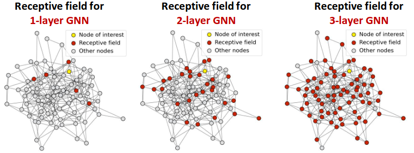
The Issue of stacking many GNN layers

• GNN suffers from the over-smoothing problem

• The over-smoothing problem: all the node embeddings converge to the same value

  • This is bad because we want to use node embeddings to differentiate nodes
  • If two nodes have highly-overlapped receptive fields, then their embeddings are highly similar

  cs224w - lecture 5. slide

What do we learn from the over-smoothing problem?

• Be cautious when adding GNN layers
  • Step 1: Analyze the necessary receptive field to solve your problem.
  • Step 2: Set number of GNN layers $L$ to be a bit more than the receptive field we like. Do not set $L$ to be unnecessarily large!

How to enhance the expressive power of a GNN, if the number of GNN layers is small?

• We can make aggregation / transformation become a deep neural network!
• Add layers that do not pass messages (A GNN does not necessarily only contain GNN layers)
  • Pre-processing layers: Important when encoding node features is necessary.
    E.g., when nodes represent images/text
  • Post-processing layers: Important when reasoning / transformation over node embeddings are needed
    E.g., graph classification, knowledge graphs

What if my problem still requires many GNN layers?

• Add skip connections in GNNs

  • Keys: Node embeddings in earlier GNN layers can sometimes better differentiate nodes

  • Solution: We can increase the impact of earlier layers on the final node embeddings, by adding shortcuts in GNN

  • $F(\rm x) + x$

  • Skip connections create a mixture of models. ($N$ skip connections → $2^N$ possible paths)

  • We automatically get a mixture of shallow GNNs and deep GNNs

    

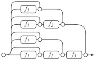
  • Other options: Directly skip to the last layer

Why need to manipulate graphs?

• Our assumption so far has been: Raw input graph = Computational graph

Reasons for breaking this assumption.

• Feature level:
  • The input graph lacks features $\rarr$ feature augmentation
  • Certain structures are hard to learn by GNN (ex. cycle)
• Structure level:
  • The graph is too sparse (Inefficient message passing)
    $\rarr$ Add virtual nodes / edges
    • Suppose in a sparse graph, two nodes have shortest path distance of 10.
    • After adding the virtual node, all the nodes will have a distance of 2
      (Node A – Virtual node – Node B)
      $\rarr$ Greatly improves message passing in sparse graphs
  • The graph is too dense (Message passing is too costly)
    $\rarr$ Sample neighbors when doing message passing
  • The graph is too large (Cannot fit the computational graph into a GPU)
    $\rarr$ Sample subgraphs to compute embeddings