• CS224W: Machine Learning with Graphs

How Expressive are GNNs?#

• Recap a GNN Layer

  $\begin{aligned}
  {\rm m}_u^{(l)} &= \text{\small MSG}^{(l)}({\rm h}_u^{(l-1)}), u \in \{N(v)\cup v\}\\
  {\rm h}_v^{(l)} &= \text{\small AGG}^{(l)}(\{{\rm m}_u^{(l)},u\in N(v)\}, {\rm m}_v^{(l)})
  \end{aligned}$

Expressive Power of GNNs#

We use node same/different colors to represent nodes with same/different features.

Local Neighborhood Structures#

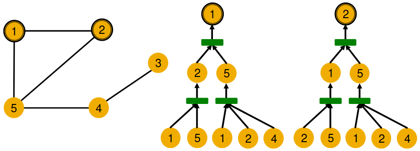
They are symmetric within the graph.

• Node 1 has neighbors of degrees 2 and 3.
• Node 2 has neighbors of degrees 2 and 3.

And even if we go a step deeper to 2nd hop neighbors, both nodes have the same degrees (Node 4 of degree 2)

But GNN only sees node features (not IDs):

• A GNN will generate the same embedding for nodes 1 and 2 because:
  • Computational graphs are the same.
  • Node features (colors) are identical.

In general, different local neighborhoods define different computational graphs

GNN’s node embeddings capture rooted subtree structures.

Expressive GNNs should map subtrees to the node embeddings injectively.

Key observation: Subtrees of the same depth can be recursively characterized from the leaf nodes to the root nodes.

If each step of GNN’s aggregation can fully retain the neighboring information, the generated node embeddings can distinguish different rooted subtrees.

In other words, most expressive GNN would use an injective neighbor aggregation function at each step.

Computational graph = Rooted subtree

Key observation: Expressive power of GNNs can be characterized by that of neighbor aggregation functions they use.

• A more expressive aggregation function leads to a more expressive a GNN.

Neighbor Aggregation#

• GCN (mean-pool), Kipf and Welling, ICLR 2017

  Element-wise mean pooling + Linear + ReLU non-linearity

  • GCN’s aggregation function cannot distinguish different multi-sets with the same color proportion. - Theorem [Xu et al. ICLR 2019] → not injective

• GraphSAGE (max-pool), Hamilton et al., NeurIPS 2017

  MLP + element-wise max-pooling

  • GraphSAGE’s aggregation function cannot distinguish different multi-sets with the same set of distinct colors. - Theorem [Xu et al. ICLR 2019] → not injective

Graph Isomorphism Network (GIN)#

Proof Intuition#

$\Phi\left(\sum_{x\in S} f(x) \right)$

$\Phi$ and $f$ are some non-linear functions.

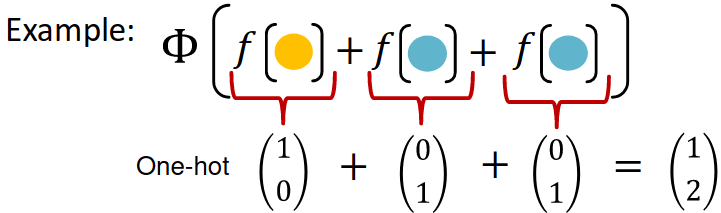
$f$ produces one-hot encodings of colors. Summation of the one-hot encodings retains all the information about the input multi-set.

Universal Approximation Theorem [Hornik et al., 1989]

• 1-hidden-layer MLP with sufficiently-large hidden dimensionality and appropriate non-linearity $\sigma(\cdot)$(including ReLU and sigmoid) can approximate any continuous function to an arbitrary accuracy.

$\text{\small MLP}_\Phi\left(\sum_{x\in S} \text{\small MLP}_f (x)\right)$

the full model of GIN by relating it to WL graph kernel (traditional way of obtaining graph-level features).

Any injective function over the tuple, $(c^{(k)}(v), \{c^{(k)}(u)\}_{u\in N(v)})$

can be modeled as

$\text{\small MLP}_\Phi\left((1+\epsilon)\cdot \text{\small MLP}_f (c^{(k)}(v)) + \sum_{u\in N(v)} \text{\small MLP}_f (c^{(k)}(u)) \right)$

$\epsilon$ is a learnable scalar.